Example 1: Two plants, constant supply curves
This example shows the application of SymEnergy to a system with
- two time slots
- two power plants
- storage capacity
Power plant cost supply curves are constant. A similar example was discussed in detail in https://doi.org/10.1016/j.eneco.2019.104495
On the technical side, this example demonstrates the adjustment of model parameters at various stages.
Jupyter Notebook available on github: https://github.com/mcsoini/symenergy/blob/master/examples/example_constant.ipynb
Model initialization
- The model structure is initialized. See the documentation section Add model components for further details on their parameters and initialization.
- Parameter values (
load,vre,vc0,capacityetc.) are insignificant at this stage as long as they are!=None. They represent default values and define the model structure. - m.generate_solve()` loads the solved model results from the corresponding pickle file if a model with the same structure (variables and multipliers) was solved earlier. The method call
m.cache.delete()would delete this file and forces the model to re-solve. nthreadis the number of cores used for parallelized solving using Python’s multiprocessing.curtailment=Trueadds curtailment variables to each of the model’s time slots.- Storage operation is limited to day-time charging and night-time discharging, as defined by the
slots_mapparameter (see Storage).
Example results
The model attribute m.df_comb is a DataFrame containing all mathematically feasible solutions of the optimization problem. It is indexed by the constraint combinations (columns act_… and idx).
For any existing index idx we can print the results for each variable using the convenience function m.print_results:
**************** curt_p_day ****************
0
**************** curt_p_night ****************
0
**************** g_p_day ****************
0
**************** g_p_night ****************
eff_phs_none**1.0*(l_day - vre_day*vre_scale_none) + l_night - vre_night*vre_scale_none
**************** lb_curt_pos_p_day ****************
eff_phs_none**0.5*w_none*(ec_phs_none - eff_phs_none**0.5*vc0_g_none)
**************** lb_curt_pos_p_night ****************
-vc0_g_none*w_none
**************** lb_g_pos_p_day ****************
w_none*(-ec_phs_none*eff_phs_none**0.5 + eff_phs_none**1.0*vc0_g_none - vc0_g_none)
**************** lb_n_pos_C_ret_none ****************
fcom_n_none
**************** lb_n_pos_p_day ****************
w_none*(-ec_phs_none*eff_phs_none**0.5 + eff_phs_none**1.0*vc0_g_none - vc0_n_none)
**************** lb_n_pos_p_night ****************
w_none*(vc0_g_none - vc0_n_none)
**************** n_C_ret_none ****************
0
**************** n_p_day ****************
0
**************** n_p_night ****************
0
**************** phs_e_none ****************
eff_phs_none**0.5*w_none*(-l_day + vre_day*vre_scale_none)
**************** phs_pchg_day ****************
-l_day + vre_day*vre_scale_none
**************** phs_pdch_night ****************
eff_phs_none**1.0*(-l_day + vre_day*vre_scale_none)
**************** pi_phs_pwrerg_chg_none ****************
ec_phs_none - eff_phs_none**0.5*vc0_g_none
**************** pi_phs_pwrerg_dch_none ****************
eff_phs_none**0.5*vc0_g_none
**************** pi_supply_day ****************
eff_phs_none**0.5*(-ec_phs_none + eff_phs_none**0.5*vc0_g_none)
**************** pi_supply_night ****************
vc0_g_none
This constraint combination corresponds the combination of active and inactive constraints shown below:
- The power output from the plant n is zero (
act_lb_n_pos_p_day == True,act_lb_n_pos_p_night == True) - The capacity retirement of n is zero (
act_lb_n_pos_C_ret_none == True) - Consequently, none of the n capacity constraints are binding.
- Day-time power production from g us zero (
act_lb_g_pos_p_day == True) - Storage operation is non-zero (
act_lb_phs_pos_... == False) and not capacity-constrained (act_lb_phs_..._cap_... == False) - Curtailment is zero during both time slots (
act_lb_curt_pos_p_... == True)
act_lb_n_pos_p_day              True
act_lb_n_pos_p_night            True
act_lb_n_pos_C_ret_none         True
act_lb_n_p_cap_C_day           False
act_lb_n_p_cap_C_night         False
act_lb_n_C_ret_cap_C_none      False
act_lb_g_pos_p_day              True
act_lb_g_pos_p_night           False
act_lb_phs_pos_pchg_day        False
act_lb_phs_pos_e_none          False
act_lb_phs_pos_pdch_night      False
act_lb_phs_pchg_cap_C_day      False
act_lb_phs_pdch_cap_C_night    False
act_lb_phs_e_cap_E_none        False
act_lb_curt_pos_p_day           True
act_lb_curt_pos_p_night         True
Name: 218, dtype: object
All model parameters are gathered in the m.parameters collection. Their attributes can be accessed by calling the Parameters instance.
[('vc0_n_none', 10),
 ('fcom_n_none', 9),
 ('C_n_none', 3500),
 ('vc0_g_none', 90),
 ('l_day', 5000),
 ('vre_day', 8500),
 ('w_none', 12),
 ('l_night', 4500),
 ('vre_night', 850),
 ('ec_phs_none', 1e-12),
 ('eff_phs_none', 0.75),
 ('C_phs_none', 1),
 ('E_phs_none', 1),
 ('vre_scale_none', 1)]
Similarly, constraints and their expressions are stored in instances of the Variables class (of the model and the components). For example, the storage’s inequality constraint names, multiplier symbols, and expressions can be accessed as follows:
[('phs_pos_pchg_day', lb_phs_pos_pchg_day, phs_pchg_day),
 ('phs_pos_e_none', lb_phs_pos_e_none, phs_e_none),
 ('phs_pos_pdch_night', lb_phs_pos_pdch_night, phs_pdch_night),
 ('phs_pchg_cap_C_day', lb_phs_pchg_cap_C_day, -C_phs_none + phs_pchg_day),
 ('phs_pdch_cap_C_night',
  lb_phs_pdch_cap_C_night,
  -C_phs_none + phs_pdch_night),
 ('phs_e_cap_E_none', lb_phs_e_cap_E_none, -E_phs_none + phs_e_none)]
Evaluation
The closed-form analytical solutions are evaluated for selected combinations of parameter values. This allows to
- plot the results
- identify relevant constraint combinations
Adjustment of model parameters
Model parameters can be freely adjusted prior to the symenergy.evaluator.Evaluator initialization. Here we set the total VRE production to 100% of the total load. This fixed VRE production profile is scaled below using the internal vre_scale model parameter.
Initialize evaluator instance and define model parameter values
The x_vals argument defines for which parameter values the solutions are evaluated. For each value combination the optimal constraint combination is identified.
The ev.get_evaluated_lambdas_parallel() call generates a DataFrame df_lam_func attribute which contains functions for each model variable and constraint combination. These functions only depend on the parameters defined by the x_vals argument. As an example, the daytime charging power under constraint combination 3330 can be printed as follows:
def _98610945ede4c0de22cac7687d8a3aa3(vre_scale_none,C_phs_none,E_phs_none,eff_phs_none,C_n_none):
    return((1/12)*E_phs_none*eff_phs_none**(-0.5))
Definition of interdependent parameter values
The ev.df_x_vals attribute corresponds to the table constructed from all combinations of parameter values defined in the x_vals attribute:
| vre_scale_none | C_phs_none | E_phs_none | eff_phs_none | C_n_none | |
|---|---|---|---|---|---|
| 0 | 0.0 | 0.0 | None | 0.75 | 2000 |
| 1 | 0.0 | 0.0 | None | 0.75 | 4000 |
| 2 | 0.0 | 0.0 | None | 0.75 | 5000 |
| 3 | 0.0 | 0.0 | None | 0.90 | 2000 |
| 4 | 0.0 | 0.0 | None | 0.90 | 4000 |
The functions in the ev.df_lam_func table are evaluated for each of these table’s rows. Prior to this evaluation, the df_x_vals table can be modified. This allows to
- filter irrelevant parameter combinations
- define certain logically connected parameter values. In this example, two types of storage are considered:
- high efficiency (90%) storage with small discharge duration of (4 hours)
- storage with lower round-trip efficiency (75%) but higher energy capacity (14 hours duration)
   vre_scale_none  C_phs_none  E_phs_none  eff_phs_none  C_n_none
0             0.0         0.0         0.0          0.75      2000
1             0.0         0.0         0.0          0.75      4000
2             0.0         0.0         0.0          0.75      5000
3             0.0         0.0         0.0          0.90      2000
4             0.0         0.0         0.0          0.90      4000
5             0.0         0.0         0.0          0.90      5000
6             0.0      2500.0     35000.0          0.75      2000
7             0.0      2500.0     35000.0          0.75      4000
8             0.0      2500.0     35000.0          0.75      5000
9             0.0      2500.0     10000.0          0.90      2000
Length:  252
Evaluate results for all entries of the Evaluator.df_x_vals table
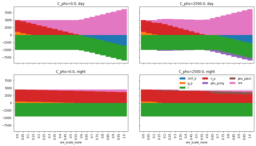
Simple energy balance plot with and without storage for day and night
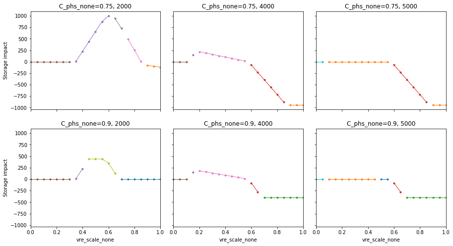
Impact of storage on baseload production by constraint combination
Using a slightly more involved analysis the impact of storage on the production from baseload plants can be plotted. The data series correspond to the least-cost constraint combinations which are active for certain parameters.